
Stress-strain data is fundamental to the analysis of structures since important decisions related to failure and integrity of structures are based on this data and on material properties derived from this data. Therefore, it is very important that engineers have a good grasp of engineering material properties as well as how to convert test data from a mechanical testing device into stress strain curves useful for design and analysis. Additionally, it is shown how to interpret and transform this data for finite element analysis applications involving large plastic deformations.
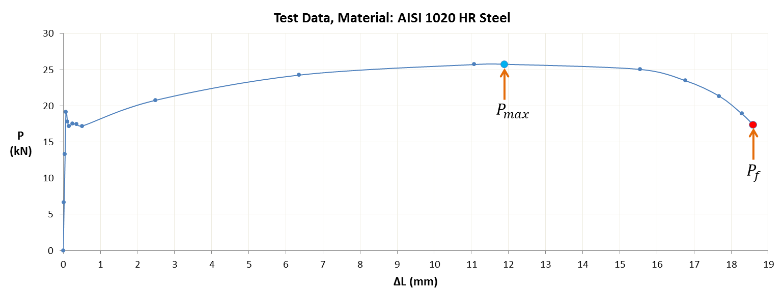
Typically, mechanical testing involves a tension test of a circular cross section rod specimen. As the machine pulls the rod in tension, the applied force P is measured along with length extension. A typical test data of steel specimen is shown below. The highest force reached during testing indicated by the blue dot whereas the red dot is the point of fracture.
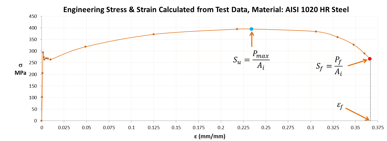
This data is converted into what is known as engineering stress and strain plot as using:
![]()
Where ‘Ai’ and ‘Li’ are initial cross section area and gage length of the specimen. Note that there is a sharp bump at the end of the linear region which is very typical of some metals in particular low-carbon steels. After the bump, the engineering stress-strain curve rises up to the maximum stress also known as ultimate tensile strength or ‘Su’. This rise up to Su is known as strain hardening as the material is increasing its resistance to strain. The Engineering stress-strain chart is shown below:
Material Properties Derived from Engineering Stress-Strain Data
Young’s Modulus ‘E’
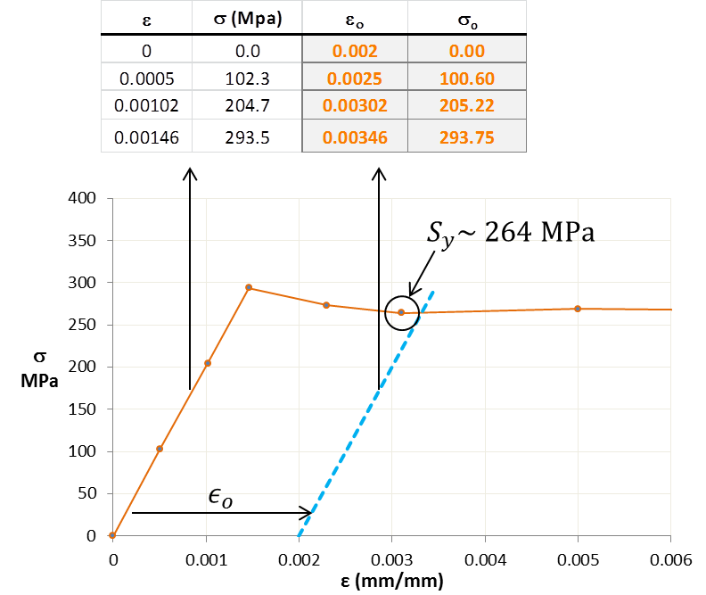
To obtain Young’s modulus, a least square fit is carried on the linear portion of the engineering stress-strain plot in order to obtain the slope ‘E’. As shown in the zoomed in linear region of stress-strain curve below, the first four data points on the linear portion are used in order to obtain a least square fit of a straight line which is then used to compute the slope or modulus E.
Yield Strength ‘Sy’
The yield strength is calculated by offsetting the original strain data by 0.002 as shown in the third column in the figure above. The stress in the fourth column is obtained by simply multiplying the offset strain by modulus E. The intersection of the shifted (blue dotted line) with engineering stress-strain curve gives the yield strength. In this case, I have used the nearest data point (shown encircled) to the intersection to obtain the yield strength of ~ 264 MPa. This is also known as offset yield strength. The offset yield method allows us to go past the sharp bump at the end of the linear portion of stress-strain curve.
Ultimate Tensile Strength ‘Su’
The ultimate tensile strength is basically the maximum engineering stress on the stress-strain curve.
Engineering Fracture Strength ‘Sf’
This is obtained from force at fracture as shown in the engineering stress-strain chart above. In brittle materials Su ~ Sf where as in ductile material Su > Sf.
Strain Hardening Ratio
This is defined as Su/Sy i.e. ultimate strength over yield strength. This ratio can range from 1.1 to 1.4 in metals.
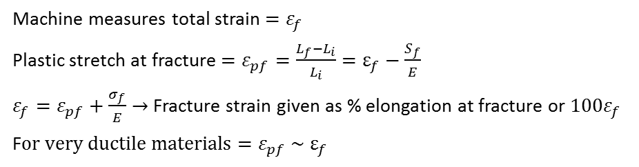
Measure of Ductility
Ductility is the ability to stretch by plastic strain up to fracture. After strain hardening, the material goes into necking phase as shown below all the way to fracture. When metal finally breaks at Sf, the elastic stretch between atomic bonds goes away and so the test specimen actually shrinks and recovers elastic part of the strain. The stretched length of the test specimen after fracture is Lf. The machine measures the total deformation up to fracture which includes elastic + plastic strain at fracture. Therefore, the fracture strain is also known as % elongation at fracture. Another measure of ductility is the % reduction in area or % RA. These terms are explained mathematically:
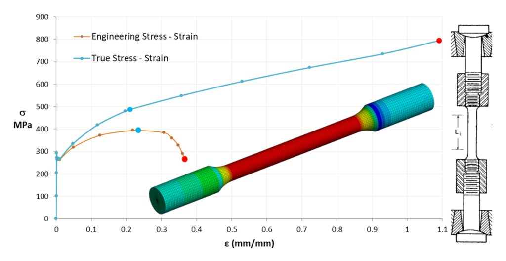
True Stress and Strain
Engineering stress and strain are applicable for small strains where test specimen dimensional changes are negligible. For large strains, in particular, finite element simulations of nonlinear plasticity phenomena, true stress and strain definitions must be used These are shown in the chart below.
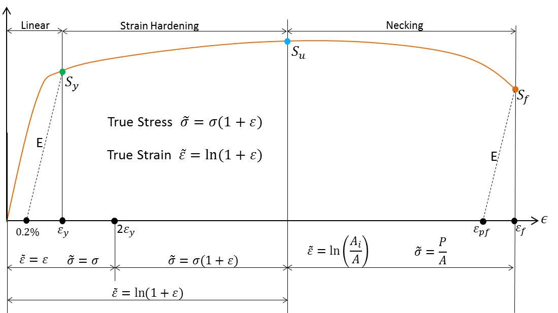
It also shows that true stress and strain are applicable up to ultimate tensile strength. Once necking starts, the true stress and strains can only be computed if actual cross section areas are measured during testing. The formulations beyond ultimate stress are also shown. Also, note that the true stress and strain are nearly equal to the engineering counterparts up to 2x yield strain. The true stress formula is not valid below 2x yield point (roughly).
Example of Material Data Extraction From Test Data
The table below shows a step by step process of how to get from test data to engineering and true stress strain curves as explained above.
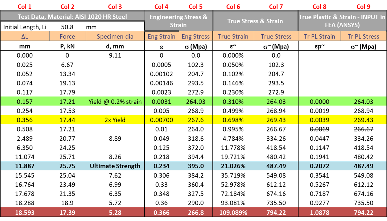
The first three columns is the test data from mechanical testing machine (Note: Data from actual testing of AISI HR 1020 steel specimen) . The third column shows specimen diameter measured during the test at some discrete applied loads. The test specimen initial length and diameter are also shown.
The next two columns (4 & 5) show engineering strain and stress calculated from test data. Columns 6 & 7 show true strain and stress computed from columns 4 & 5 using formulas shown above.
Note that the true strain in column 7 is the total strain. For FEA computation, we need to provide true plastic strain corresponding to true stress data as nonlinear material property. This means taking the true strain value at yield (green row, Col 6) which is entirely elastic and subtracting it from the entire column 6 to generate the plastic strain shown in column 8. Column 9 is simply a copy of column 7 but the stress starts from zero plastic strain. The data in columns 8 and 9 is ready to be used in nonlinear material models in commercial packages like ANSYS. Note that plastic stress (column 9) should be monotonically increasing as required by ANSYS. Hence one of the data points violating this rule is crossed out.
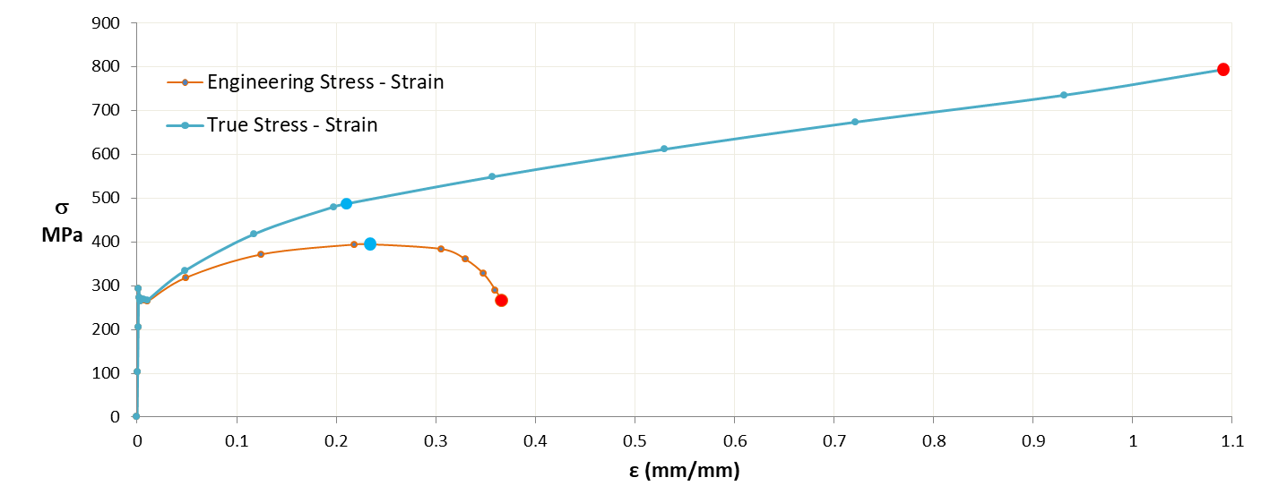
As a comparison, the engineering and true stress strain data is shown below. The large blue dot represents ultimate stress and red dot at the end is fracture or failure of specimen.
FE Based Virtual Test
A finite element based virtual mechanical test can be carried out in order to replicate the behaviour of real physical test by using the derived material properties shown above and comparing the output with original test data.
For this purpose, an axisymmetric FE model is created with boundary conditions simulating the grip in mechanical testing machine. Simulated test is shown below:
If you observe carefully, you can see a reduction in speciment diameter due to elongation just like the physical specimen. The chart shown below compares FE output with experimental data.
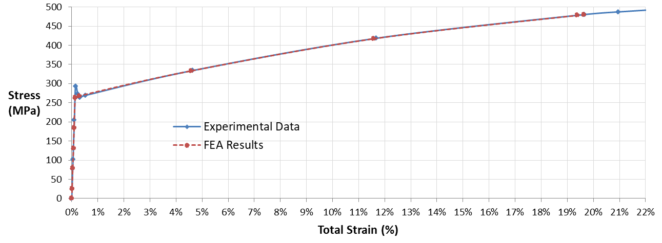
Maximum axial stress vs total strain comparison of FE output with experimental data.
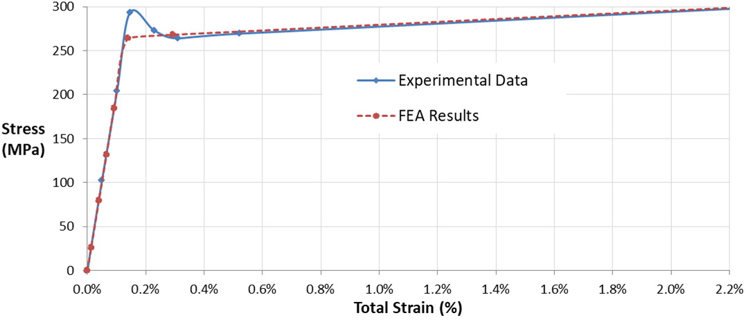
The zoomed in version of the above chart shows how initial yield bump is missing in FE output due to the 0.2% strain shift used in evaluating yield strength and bypassing that bump as explained above.
Finally, a comparison of test specimen diameter is shown below
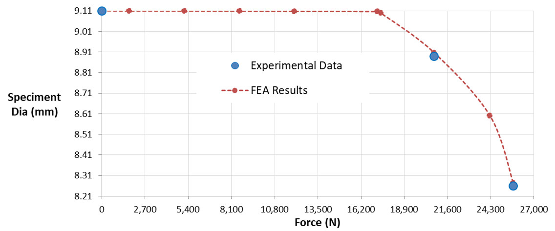
These charts show that we can replicate actual mechanical testing in FE by utilizing phyical test data in FE simulation. I’ll have more on this in later articles as we explore nonlinear material behavior including load cycling and fatigue in detail.

2 Comments
I believe there a two small mistakes in this otherwise very informative post.
1. Under section “Yield strenght ‘Sy'” you say “The stress in the fourth column is obtained by simply multiplying the offset strain by modulus E.”. However, the fourth column seems to be the multiplication of the original (and thus non-offset) strain values by the Young’s Modulus. I believe this is the correct solution, but the wrong description.
2. Under section “Measure of Ductility” following formula is given: ε_pf = (L_f – L_i)/L_i. In this formula I assumed that ε_pf is the plastic strain at the point of fracture, L_f is the total length at the point of fracture and L_i is the initial length. Isn’t this then the formula for ε_f aka the strain at the point of fracture? Or should it be L_pf instead of L_f to denote the plastic part?
Jonas,
Thanks for noting these. I’ll go through the article again and revise it as needed.
ZK